2. Tensor Operation & Minibatch
In the field of deep learning, the tensor is like a multi-dimension numerical array.
- 0-dim: scalar
- 1-dim: vector
- 2-dim: matrix
- n-dim: general tensor
Tensors are fundamental because they allow data to be represented and processed efficiently in any number of dimensions. In Python, tensors are often represented with NumPy array or framework-specific tensor objects such as those in PyTorch or TensorFlow.
Using tensors is simpler and faster than using explicit loops.
- The Python interpreter and underlying libraries can process tensor operations much more efficiently than iterative approaches.
- On GPUs, tensor operations benefit from parallelization, leading to significant performance improvements.
Generally in deep learning, a minibatch refers to processing multiple data samples at once through a neural network.
-
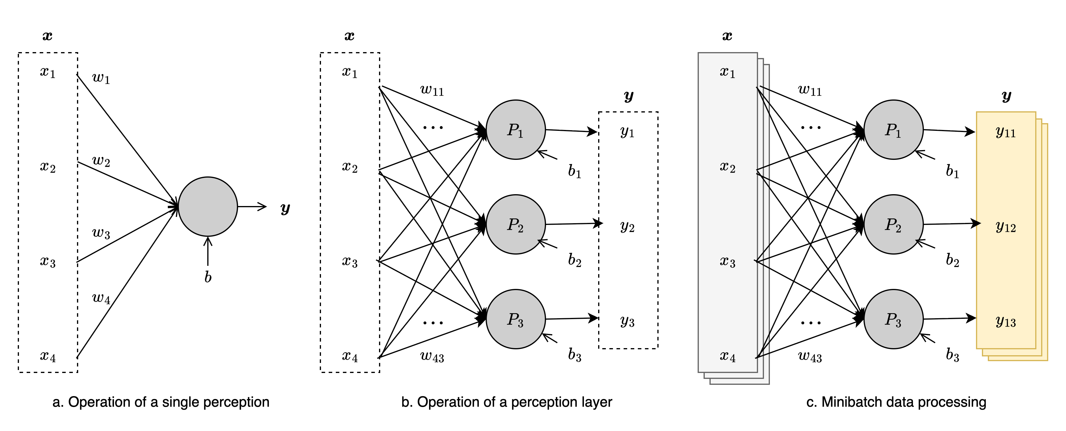
a is the operation of a single perceptron. This perceptron computes a scalar output:
$$ y=x_{1}w_{1} + \cdots + x_{n}w_{n} + b = \boldsymbol{xw} + b $$
- weight vector: $\boldsymbol{w}=(w_{1},\ \dots \ , \ w_{n})$
- input vector: $\boldsymbol{x}=(x_{1},\ \dots \ , \ x_{n})$
- scalar bias: $b$
- It is possible to compute $y$ by summing all $x_{i}w_{i}$ terms in a loop, but using the dot product of vectors is much more efficient.
Linear Operation: An operation that can be expressed as a linear function of the inputs.
Nonlinear Operation: An operation that cannot be expressed as a linear function of the inputs.
-
b shows how a layer of perceptrons processes a single input vector:
$$ y_{i}=x_{1}w_{i1} + \cdots +x_{n}w_{in} + b = \boldsymbol{xw_{i}} + b_{i} $$
- weight matrix: $\boldsymbol{W}$
- bias vector: $\boldsymbol{b}$
In matrix form, this is written as:
$$ \boldsymbol{y} = \boldsymbol{xW} + \boldsymbol{b} $$
Using this matrix expression is much more efficient than computing each perceptron with explicit loops.
-
c illustrates the operation of a perceptron layer under minibatch processing:
-
Multiple input samples are collected.
- input matrix: $X$
- output matrix: $Y$
-
The same process as in b is applied to each sample:
$$ \boldsymbol{y_{j}} = \boldsymbol{x_{j}}W + \boldsymbol{b} $$
-
Collectively, the minibatch process can be expressed as:
$$ \boldsymbol{Y} = \boldsymbol{XW} + \boldsymbol{b} $$ Using matrix operations is much easier and more efficient than computing each case with loops, as in a and b.
-
This demonstrates how neural network computations scale from a single perceptron to full layers and minibatches, forming the foundation of deep learning models.